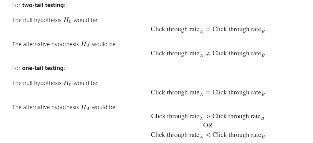
A/B Testing
A/B Testing is a controlled experiment that is used to examine whether the changes that we made to a product/web service have significant influences. For each A/B testing, we would have a controlled version A and a variant version B. We want to test whether changing from A to B makes a difference.
A/B testing is essentially hypothesis testing in Statistics. Hypothesis testing has two hypotheses. The null hypothesis is the fact that we are not interested in, which is changing from A to B does not make a difference. The alternative hypothesis is the fact that we care about, which would be changing from A to B does make a difference.
General Process for conducting A/B Testing
The process of conducting A/B testing is like conducting an experiment.
1. First, we should define the goal of this A/B testing. Hence, we would need to decide the metrics we would like to use in the A/B testing. There are two different types of metrics, discrete and continuous.
- Discrete metrics have only two states (0 or 1, True or False, Yes or No and etc). For example, if we are conducting A/B testing, we could have the following discrete metrics:
- Click through rate: if a new version of button is introduced to the website, do users click on it or not? The goal for this metric could be a 2% increase in click through rate after changing from version A to version B.
- Retention rate: if a new feature is added to the web service, do users continue to log in to the website after a number of days? The goal for this metric could be a 2% increase in retention rate after changing from version A to version B.
- Continuous metrics have more than two states and are continuous values. For example, we could have the following continuous metrics:
- Daily active users: how many active users per day? The goal for this metric could be 10 more daily active users after changing from version A to version B.
- Average duration: how long does an user stay on a website? The goal for this metric could be 2 more minutes of duration after changing from version A to version B.
2. Next, we should create the variant for A/B Testing
There are various things we can do for A/B testing. For example, to change a color of a button on the website, to introduce a different advertisement on the landing page and etc.
3. Generating hypotheses
Assuming we are using Click through rate as a metric.
4. Calculate Minimum Sample Size (if applicable)
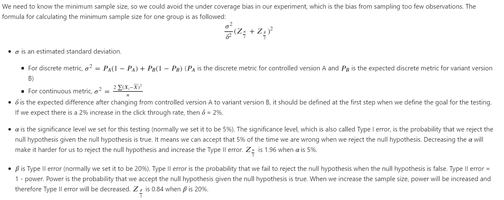
We should notice from the minimum sample size formula that larger difference would require a smaller sample size for detection while a smaller difference would require a larger sample size.
5. Calculate the test duration

6. Start the experiment
We have defined the goal, created controlled version and variant version, calculated the minimum sample size and test duration, it is now the time to start the experiment. To ensure there is no sampling biases in our testing (which means the sample is indeed the true representation of the population), we should use random sampling method to randomly assign people to the controlled group or the variant group.
However, we should also be aware of the Simpson’s paradox. Simpson’s paradox is a phenomenon that there is an effect when two groups are combined while the effect disappears or reverses when two groups are separated. Simpson’s paradox is caused by confounders, which are variables that are both correlated to the dependent variable/target and independent variables. For example, if we want to predict housing prices (dependent variable) based on four independent variables, namely the size of the house, the number of bedrooms the house has, the age of the house and the location. In this task, the size of the house is both associated with the number of bedrooms and the housing price. Larger the size of the house, more bedrooms and higher housing price. To avoid the Simpson’s paradox, we should control the confounder by applying stratification to our sample, which means stratifies (separates) our samples based on the confounder, such as splitting the sample into female or male. We could also include blocking into our testing to improve the accuracy.
7. Collect data
After the experiment starts, we would need to collect the data that is of our interest based on the metric that we chose, such as whether the user click on the button when they visit the website, or the number of active users every day.
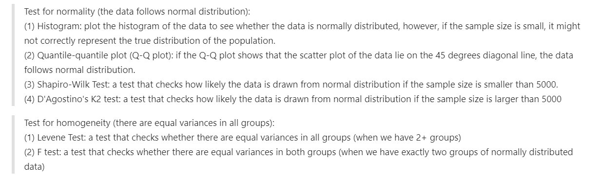
8. Choosing a right test
After the experiment is done and we finish collecting the experiment data, we need to determine the test that is appropriate to our data. For A/B testing, there are various tests that we could use.
- Discrete metrics:
- Large sample size: Chi-squared test which tests the correlation between categorical variables
- Small sample size: Fisher’s exact test which tests the correlation between categorical variables
- Continuous metrics:
- Appropriate situations to use Z-test:
- Large sample size and known variances
- Small sample size and normality is satisfied and known variances
- Appropriate situations to use student’s t-test:
- Large sample size and unknown variances and homogeneity is satisfied
- Small sample size and normality is satisfied and unknown variances and homogeneity is satisfied
- Appropriate situations to use Welch’s t-test:
- Large sample size and unknown variances and homogeneity is not satisfied
- Small sample size and normality is satisfied and unknown variances and homogeneity is not satisfied
- Appropriate situations to use Mann–Whitney U test:
- Small sample size and normality is not satisfied
- Appropriate situations to use Z-test:
9. Calculate p-value
After selecting the appropriate test, we should calculate the test statistic. The formula for test statistic would depend on the test that we choose. After calculating the test statistic, we could calculate the p-value.
p-value is the probability that the test statistic is at least as extreme as the observed data, given the null hypothesis is true. Or we could say the p-value is the probability that our observed data occurs by chances given the null hypothesis is true.
10. Draw the conclusion

Example
Business problem
The dataset is taken from Kaggle at https://www.kaggle.com/yufengsui/datacamp-project-mobile-games-a-b-testing/notebook. Please find the introduction of the business problem below:
“Cookie Cats is a hugely popular mobile puzzle game developed by Tactile Entertainment. This project is based on a mini project from Datacamp. As players progress through the levels of the game, they will occasionally encounter gates that force them to wait a non-trivial amount of time or make an in-app purchase to progress. In addition to driving in-app purchases, these gates serve the important purpose of giving players an enforced break from playing the game, hopefully resulting in that the player’s enjoyment of the game being increased and prolonged. But where should the gates be placed? Initially the first gate was placed at level 30. In this project, we’re going to analyze an AB-test where we moved the first gate in Cookie Cats from level 30 to level 40.”
Import the data and necessary packages
import numpy as np
import pandas as pd
import plotly.express as px
import matplotlib.pyplot as plt
from scipy import stats
import statsmodels.api as sm
%matplotlib inline
data = pd.read_csv("../cookie_cats.csv")
Exploratory Data Analysis
data.head()
| userid | version | sum_gamerounds | retention_1 | retention_7 | |
|---|---|---|---|---|---|
| 0 | 116 | gate_30 | 3 | False | False |
| 1 | 337 | gate_30 | 38 | True | False |
| 2 | 377 | gate_40 | 165 | True | False |
| 3 | 483 | gate_40 | 1 | False | False |
| 4 | 488 | gate_40 | 179 | True | True |
data.info()
<class 'pandas.core.frame.DataFrame'>
RangeIndex: 90189 entries, 0 to 90188
Data columns (total 5 columns):
 #   Column          Non-Null Count  Dtype
---  ------          --------------  -----
 0   userid          90189 non-null  int64
 1   version         90189 non-null  object
 2   sum_gamerounds  90189 non-null  int64
 3   retention_1     90189 non-null  bool
 4   retention_7     90189 non-null  bool
dtypes: bool(2), int64(2), object(1)
memory usage: 2.2+ MB
There are 90,189 players in this dataset who installed the game while the AB-test was running.

Exploration of sum_gamerounds (the number of game rounds played by the player during the first week after installation)
# look at the mean, std, quantiles of the number of game rounds played by the player during the first week after installation
data.iloc[:,[1,2]].groupby("version").describe()
| sum_gamerounds | ||||||||
|---|---|---|---|---|---|---|---|---|
| count | mean | std | min | 25% | 50% | 75% | max | |
| version | ||||||||
| gate_30 | 44700.0 | 52.456264 | 256.716423 | 0.0 | 5.0 | 17.0 | 50.0 | 49854.0 |
| gate_40 | 45489.0 | 51.298776 | 103.294416 | 0.0 | 5.0 | 16.0 | 52.0 | 2640.0 |
There are almost equal number of users in the control group (gate_30) and the test group (gate_40). The mean number of game rounds by each player is roughly 50 and there are clearly outliers in both groups. Let’s take a closer look at the distribution of both groups:
data_30 = data.query("version == 'gate_30'")
data_40 = data.query("version == 'gate_40'")
data_30.sort_values(by="sum_gamerounds",ascending=False)
| userid | version | sum_gamerounds | retention_1 | retention_7 | |
|---|---|---|---|---|---|
| 57702 | 6390605 | gate_30 | 49854 | False | True |
| 7912 | 871500 | gate_30 | 2961 | True | True |
| 43671 | 4832608 | gate_30 | 2438 | True | True |
| 46344 | 5133952 | gate_30 | 2251 | True | True |
| 87007 | 9640085 | gate_30 | 2156 | True | True |
| ... | ... | ... | ... | ... | ... |
| 40973 | 4533461 | gate_30 | 0 | False | False |
| 20880 | 2323023 | gate_30 | 0 | False | False |
| 81104 | 8981313 | gate_30 | 0 | False | False |
| 87537 | 9696981 | gate_30 | 0 | False | False |
| 81466 | 9022139 | gate_30 | 0 | False | False |
44700 rows × 5 columns
data_40.sort_values(by="sum_gamerounds",ascending=False)
| userid | version | sum_gamerounds | retention_1 | retention_7 | |
|---|---|---|---|---|---|
| 29417 | 3271615 | gate_40 | 2640 | True | False |
| 48188 | 5346171 | gate_40 | 2294 | True | True |
| 36933 | 4090246 | gate_40 | 2124 | True | True |
| 88328 | 9791599 | gate_40 | 2063 | True | True |
| 6536 | 725080 | gate_40 | 2015 | True | True |
| ... | ... | ... | ... | ... | ... |
| 68657 | 7608893 | gate_40 | 0 | False | False |
| 1988 | 214700 | gate_40 | 0 | False | False |
| 80941 | 8964492 | gate_40 | 0 | False | False |
| 29402 | 3270520 | gate_40 | 0 | False | False |
| 77280 | 8556826 | gate_40 | 0 | False | False |
45489 rows × 5 columns
To ensure that our analysis is not affected by outliers and a representative of the majority of users, we are going to exclude the outlier in the data and only keep data with sum_gamerounds smaller than or equal to 3000.
# only keep data with sum_gamerounds smaller than or equal to 3000
data_30 = data_30.query("sum_gamerounds<=3000")
px.histogram(
    data.query("sum_gamerounds<=3000"),
    x="sum_gamerounds",
    color="version",
    labels={
        "sum_gamerounds": "The number of game rounds played by the player during the first week after installation",
        "version": "Version",
    },
)
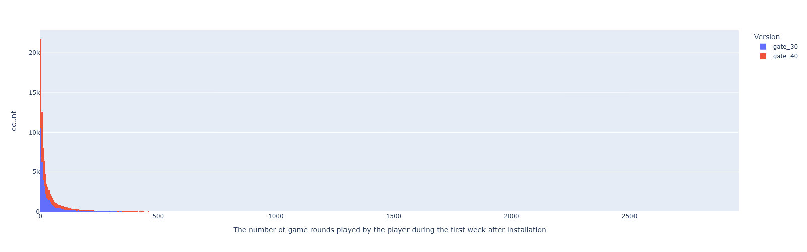
The number of game rounds appears to be heavily right skewed. Majority of players stop playing the game after roughly 150 rounds.
Exploration of retention rate
sorted_data = data.melt(
    id_vars=data.columns.tolist()[:3],
    value_vars=["retention_1", "retention_7"],
)

count_data = (
    sorted_data.iloc[:, [1, 3, 4]]
    .value_counts()
    .reset_index()
    .rename(columns={0: "count"})
)
count_data

retention_1 = (
    pd.DataFrame(
        count_data[
            (count_data["variable"] == "retention_1") & (count_data["value"] == True)
        ]
        .groupby("version")
        .sum()
        .loc[:, "count"]
        / count_data[(count_data["variable"] == "retention_1")]
        .groupby("version")
        .sum()
        .loc[:, "count"]
    )
    .reset_index()
    .rename(columns={"count": "retention_rate_after_one_day"})
)
print("The retention rate after 1 day\n")
retention_1
The retention rate after 1 day
| version | retention_rate_after_one_day | |
|---|---|---|
| 0 | gate_30 | 0.448188 |
| 1 | gate_40 | 0.442283 |
retention_7 = (
    pd.DataFrame(
        count_data[
            (count_data["variable"] == "retention_7") & (count_data["value"] == True)
        ]
        .groupby("version")
        .sum()
        .loc[:, "count"]
        / count_data[(count_data["variable"] == "retention_7")]
        .groupby("version")
        .sum()
        .loc[:, "count"]
    )
    .reset_index()
    .rename(columns={"count": "retention_rate_after_seven_days"})
)
print("The retention rate after 7 days\n")
retention_7
The retention rate after 7 days
| version | retention_rate_after_seven_days | |
|---|---|---|
| 0 | gate_30 | 0.190201 |
| 1 | gate_40 | 0.182000 |
Based on the retention rate data, gate_30 seems to be more favorable by users than gate_40.
Using the sum_gamerounds as a metric of the A/B testing
Since the sum_gamerounds is a continuous metric, we need to check the normality and possibly homogeneity if normality is satisfied to determine an appropriate test.
Check for normality
Although we can tell the data is not following the normal distribution from the histograms above, we are going to explore both Q-Q plot and Shapiro–Wilk test (sample size smaller than 5000) for further confirmation.
Q-Q plot
fig_qqplot, axes_qqplot = plt.subplots(1, 3, figsize=(15, 4), facecolor="#e5e5e5")
axes_qqplot = axes_qqplot.ravel()

for ax in axes_qqplot:
    sm.qqplot(
        data_30.sum_gamerounds, ax=axes_qqplot[0], marker="x", line="45", fit=True
    )
    sm.qqplot(
        data_40.sum_gamerounds, ax=axes_qqplot[1], marker="x", line="45", fit=True
    )
    sm.qqplot(
        data[data["sum_gamerounds"] <= 3000].sum_gamerounds,
        ax=axes_qqplot[2],
        marker="x",
        line="45",
        fit=True,
    )

axes_qqplot[0].set_title("QQ Plot for gate 30")
axes_qqplot[1].set_title("QQ Plot for gate 40")
axes_qqplot[2].set_title("QQ Plot for all data")

plt.tight_layout()
plt.show()
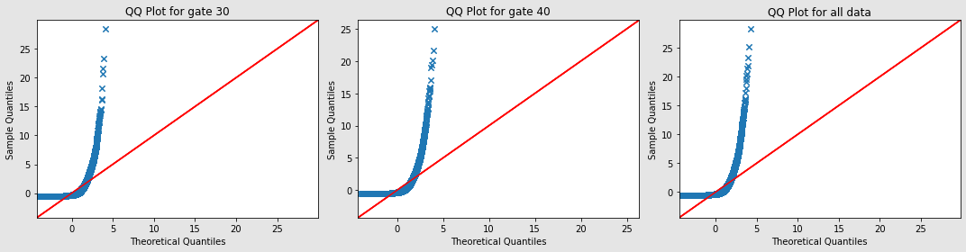
Since both groups’ scatter points are not on the 45° degree line, the data is not normally distributed for both groups.
Shapiro-Wilk Test
def normaility_check(data, alpha=0.05):
    print("Null hypothesis: the data follows normal distribution")
    print("Alternative hypothesis: the data does not follow normal distribution\n")

    test_statistic, p_value = stats.shapiro(data)

    if p_value < alpha:
        print(
            f"The p_value is {p_value}, which is smaller than the significance level of {alpha}. \nThe null hypothesis is rejected, data does not follow normal distribution"
        )
    else:
        print(
            f"The p_value is {p_value}, which is larger than the significance level of {alpha}. \nFail to reject the null hypothesis, data does follow normal distribution"
        )
print("Normaility test for data of the controlled version A\n")
normaility_check(data_30.sum_gamerounds)
Normaility test for data of the controlled version A

Null hypothesis: the data follows normal distribution
Alternative hypothesis: the data does not follow normal distribution

The p_value is 0.0, which is smaller than the significance level of 0.05.
The null hypothesis is rejected, data does not follow normal distribution
print("Normaility test for data of the variant version B\n")
normaility_check(data_40.sum_gamerounds)
Normaility test for data of the variant version B

Null hypothesis: the data follows normal distribution
Alternative hypothesis: the data does not follow normal distribution

The p_value is 0.0, which is smaller than the significance level of 0.05.
The null hypothesis is rejected, data does not follow normal distribution
Since the normality is not satisfied, we could go for Mann–Whitney U test without further checking the homogeneity.
def mann_whitneyutest(data1, data2, alpha=0.05):

    print("Null hypothesis: The two populations are equal.")
    print("Alternative hypothesis: The two populations are not equal.\n")

    test_statistic, p_value = stats.mannwhitneyu(data1, data2)

    print(f"The p-value for Mann-Whitney U test is {round(p_value, 10)}")

    if p_value < alpha:
        print(
            f"The p_value is {round(p_value, 10)}, which is smaller than the significance level of {alpha}. \nThe null hypothesis is rejected, the two populations are not equal"
        )
    else:
        print(
            f"The p_value is {round(p_value, 10)}, which is larger than the significance level of {alpha}. Fail to reject the null hypothesis.\nThe two populations are equal"
        )
mann_whitneyutest(data_30.sum_gamerounds, data_40.sum_gamerounds)
Null hypothesis: The two populations are equal.
Alternative hypothesis: The two populations are not equal.

The p-value for Mann-Whitney U test is 0.0508915528
The p_value is 0.0508915528, which is larger than the significance level of 0.05. Fail to reject the null hypothesis.
The two populations are equal
Conclusion
There is no significant change in the number of game rounds played by the player during the first week after installation after changing from the controlled version A (the first gate was placed at level 30) to the variant version B (the first gate was placed at level 40).
Using the retention rate as a metric of the A/B testing
Since the retention rate is a discrete metric and the sample size is relatively large, we are going to use the Chi-squared test. To perform the Chi-squared test, we need to construct the contingency table first.
retention1_contingency = pd.crosstab(index=data['version'], columns=data['retention_1'])
retention1_contingency
| retention_1 | False | True |
|---|---|---|
| version | ||
| gate_30 | 24666 | 20034 |
| gate_40 | 25370 | 20119 |
retention7_contingency = pd.crosstab(index=data['version'], columns=data['retention_7'])
retention7_contingency
| retention_7 | False | True |
|---|---|---|
| version | ||
| gate_30 | 36198 | 8502 |
| gate_40 | 37210 | 8279 |
def test_chisquared(contingency_table, alpha=0.05):

    print("Null hypothesis: Version and retention rate are independent")
    print("Alternative hypothesis: Version and retention rate are not independent\n")

    chisquare, p_value, degree_of_freedom, expected = stats.chi2_contingency(
        contingency_table, correction=False
    )

    print(f"The p_value for test is {p_value}")

    if p_value < alpha:
        print(
            f"The p_value is {round(p_value, 10)}, which is smaller than the significance level of {alpha}. The null hypothesis is rejected.\nVersion and retention rate are not independent"
        )
    else:
        print(
            f"The p_value is {round(p_value, 10)}, which is larger than the significance level of {alpha}. Fail to reject the null hypothesis.\nVersion and retention rate are independent"
        )
print("Performing the Chi_squared Test for retention rate after day 1:\n")
test_chisquared(retention1_contingency)
Performing the Chi_squared Test for retention rate after day 1:

Null hypothesis: Version and retention rate are independent
Alternative hypothesis: Version and retention rate are not independent

The p_value for test is 0.07440965529692188
The p_value is 0.0744096553, which is larger than the significance level of 0.05. Fail to reject the null hypothesis.
Version and retention rate are independent
print("Performing the Chi_squared Test for retention rate after day 7:\n")
test_chisquared(retention7_contingency)
Performing the Chi_squared Test for retention rate after day 7:

Null hypothesis: Version and retention rate are independent
Alternative hypothesis: Version and retention rate are not independent

The p_value for test is 0.0015542499756142805
The p_value is 0.00155425, which is smaller than the significance level of 0.05. The null hypothesis is rejected.
Version and retention rate are not independent
Conclusion
-
When we use retention rate after 1 day as a metric, the testing result suggests that there is no significant change in the retention rate after changing from the controlled version A (the first gate was placed at level 30) to the variant version B (the first gate was placed at level 40).
-
When we use retention rate after 7 days as a metric, the testing result suggests that there is a significant change in the retention rate after changing from the controlled version A (the first gate was placed at level 30) to the variant version B (the first gate was placed at level 40).
Conclusion for A/B testing
We have conducted three testings using different metrics. However, the metric should be decided before running the test and should be depended on the business goal.
-
When we use the continuous metric (sum_gamerounds: the number of game rounds played by the player during the first week after installation), the result is not significant. It suggests that changing from the controlled version A (the first gate was placed at level 30) to the variant version B (the first gate was placed at level 40) does not make a difference and the company should not make the change.
-
When we use the discrete metric (retention_1: did the player come back and play 1 day after installing), the result is not significant either. It suggests that changing from the controlled version A (the first gate was placed at level 30) to the variant version B (the first gate was placed at level 40) does not make a difference and the company should not make the change.
-
When we use the discrete metric (retention_7: did the player come back and play 7 days after installing), the result is significant. It suggests that changing from the controlled version A (the first gate was placed at level 30) to the variant version B (the first gate was placed at level 40) does make a difference. However, based on our initial data exploration, the retention rate for controlled version A is better than the variant version B. Therefore, the company still should not make the change.
Therefore, all three testings suggest the same result that the company should keep the first gate at level 30.
Reference
- https://www.kaggle.com/ekrembayar/a-b-testing-step-by-step-hypothesis-testing/notebook
- https://towardsdatascience.com/a-b-testing-a-complete-guide-to-statistical-testing-e3f1db140499
- https://machinelearningmastery.com/a-gentle-introduction-to-normality-tests-in-python/
- https://towardsdatascience.com/how-to-conduct-a-b-testing-3076074a8458
- https://www.kaggle.com/mustafacicek/a-b-testing-statistical-tests/notebook